Machine LearningIntroduction
At the highest level, the goal of
We aim to use the training data to predict given , where denotes a random variable in with distribution .
Example
Suppose that , where is the color of a banana, is the weight of the banana, and is a measure of banana deliciousness. Values of and are recorded for many bananas, and they are used to predict for other bananas whose values are known.
Do you expect the prediction function to be more sensitive to changes in or changes in ?
Solution. We would expect to have more influence on , since bananas can taste great whether small or large, while green or dark brown bananas generally taste very bad and yellow bananas mostly taste good.
Definition
We call the components of features, predictors, or input variables, and we call the response variable or output variable.
We categorize supervised learning problems based on the structure of .
Definition
A supervised learning problem is a regression problem if is quantitative () and a classification problem if is a set of labels.
We can treat the banana problem above as either a regression problem (if deliciousness is a score on a spectrum) or a classification problem (if the bananas are
Exercise
Explain how a machine learning task like image recognition fits into this framework. In other words, describe an appropriate feature space , describe in loose terms what the probability measure looks like, and describe in geometric terms what we are trying to accomplish when we define our prediction function.
Solution. We can take to be , where is the number of pixels in each image., because a grayscale image with pixels can be thought of as list of 1000 numbers in , with each component indicating the darkness of a single pixel. Let's suppose , which is a fairly typical image size for modern cameras.
The output set contains labels. For example, if we just have cat images and dog images to classify, then would be {"cat", "dog"}.
The probability mass occupies a very small portion of the million-dimensional cube, since the vast majority of possible images do not represent a cat or a dog. Furthermore, the geometry of the sets where mass is concentrated is presumably quite complex, since the set of changes which can be made to an image to preserve its "catness" or "dogness" is not straightforward to describe. See the figure to the right for a rough visual; that this visualization is necessarily strained, since the 3D cube and the million dimensional cube have very different geometric properties.
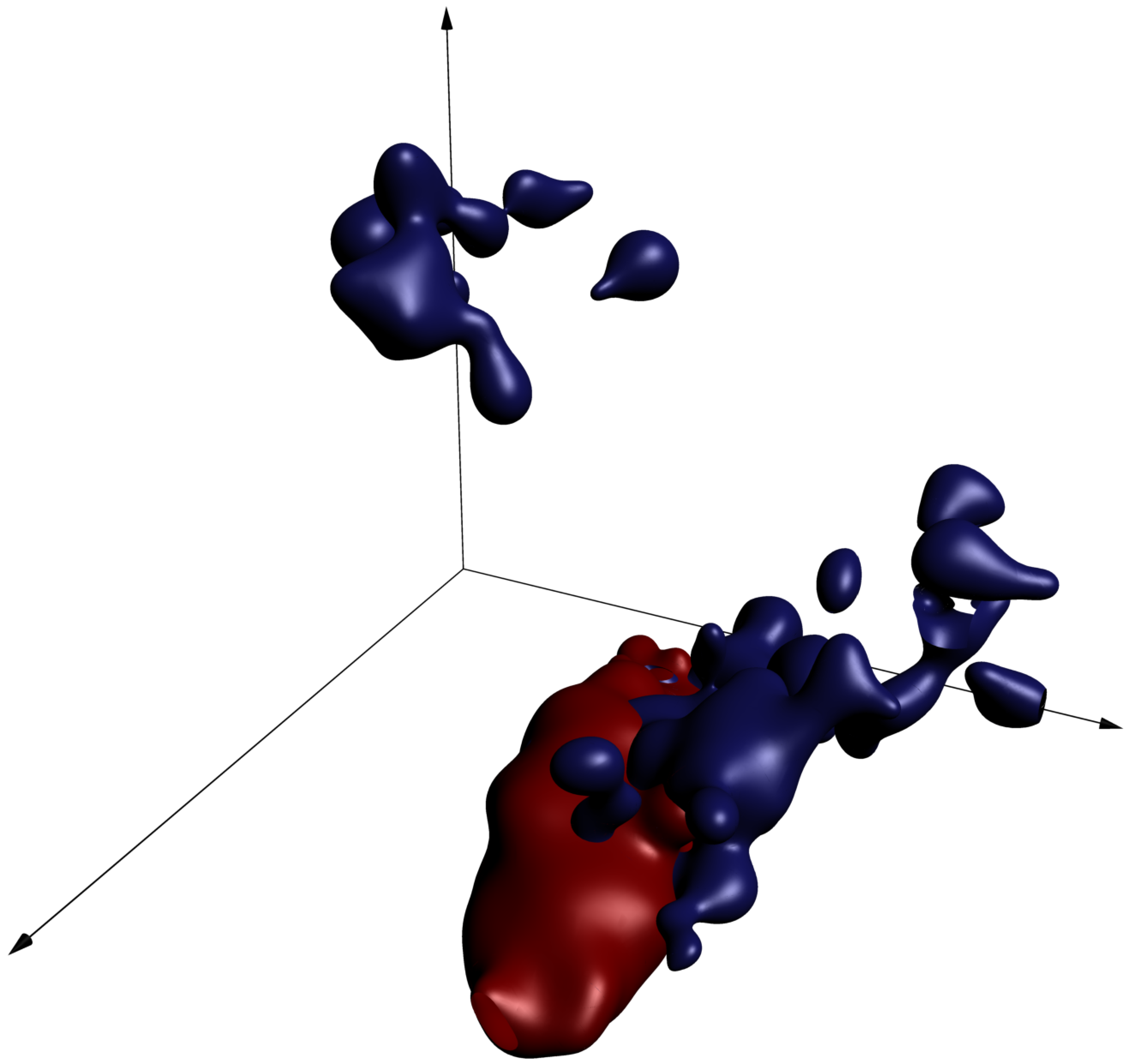
Each dimension in this figure represents a pixel darkness, and the red and blue surfaces represent level sets of the conditional probability density functions given the animal genus. Cat images are likely to fall inside the red surfaces, while dog images are more likely to fall inside the blue surfaces. This visualization should be taken with a grain of salt, since real images have many more than three pixels.
Still, one thing we can use this picture to think about is what our goal is when we're coming up with a prediction function: we should carve up the cube so as to separate the regions where there's more cat probability mass from regions where there's more dog probability mass. That way, any image of a cat or dog can be identified as "more likely a cat" or "more likely a dog".
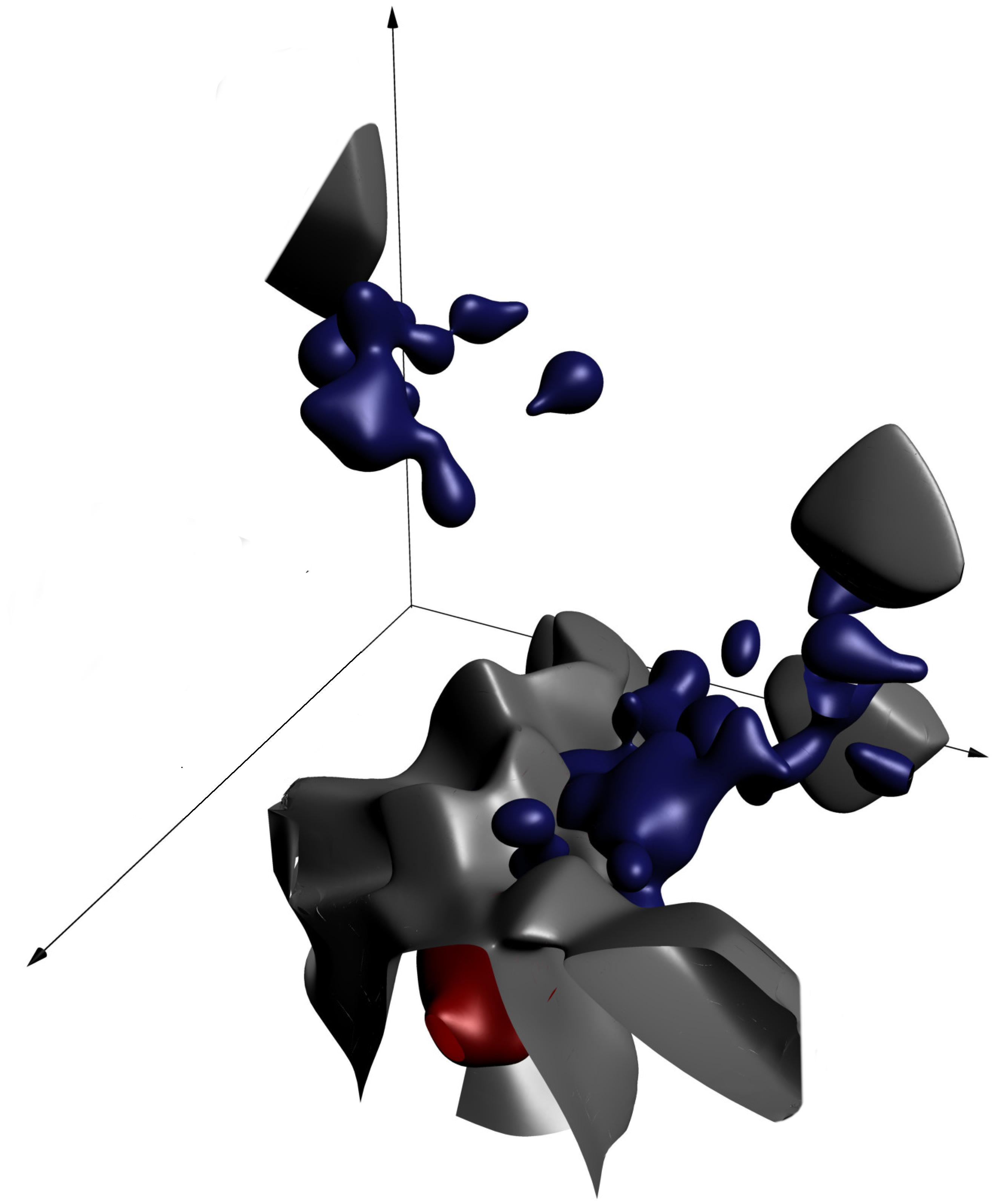
The gray surface separates regions where there's more red probability mass (for cats) from regions where there's more blue probability mass (for dogs). The goal of the prediction function is to compute whether a given point falls on the cat side or the dog side.
The loss functional
To make meaningful and unambiguous statements about a proposed prediction function , we need a rubric by which to assess it. This is customarily done by defining a loss (or risk, or error ) , with the idea that smaller loss is better. We might wish to define only for 's in a specified class of candidate functions.
Once a set of candidate functions and a loss functional are specified, a prediction function must be proposed. This can often be done the lazy way, by defining our prediction function implicitly as the function in which minimizes :
Definition
Given a statistical learning problem, a space of candidate prediction functions, and a loss functional , we define the target function to be .
(Note: argmin means the value which minimizes. So for example, is equal to 14.)
Let's look at some common loss functionals. For regression, we often use the mean squared error:
If contains the regression function , then is the target function. This is because the mean of a random variable is the constant which minimizes the expression .
Exercise
Recall the exam scores example from the KDE section of the statistics course in which we know the exact density of the distribution which generates the hours-score pairs for students taking an exam (run this cell):
using LinearAlgebra, Statistics, Roots, Optim, Plots, Random
Random.seed!(1234)

# the true regression function
r(x) = 2 + 1/50*x*(30-x)
# the true density function
σy = 3/2
f(x,y) = 3/4000 * 1/√(2π*σy^2) * x*(20-x)*exp(-1/(2σy^2)*(y-r(x))^2)

heatmap(0:0.02:20, -2:0.01:12, f,
        fillcolor = cgrad([:white, :MidnightBlue]),
        ratio = 1, fontfamily = "Palatino",
        size = (600,300), xlims = (0,20), ylims = (0,12),
        xlabel = "hours studied", ylabel = "score")

scatter!([(5,2), (5,4), (7,4), (15,4.5), (18, 4), (10,6.1)],
         markersize = 3, label = "observations")

plot!(0:0.02:20, r, label = "target function",
      legend = :topleft, linewidth = 2)
(a) What must be true of the class of candidate functions in order for the target function to be equal to the regression function ?
(b) Suppose we collect six observations, and we get the six data points shown in the plot above. Can the loss value of the prediction function plotted be decreased by lowering its graph a bit?
Solution. (a) The class of candidate functions must contain . For example, it might consistnt of all quadratic functions, or all differentiable functions. If it only contained linear functions, then the target function would be different from the regression function.
(b) No, the loss value of the prediction function depends on the actual probability measure, not on training observations. If we know the probability measure, then we have the best possible information for making future predictions, and we can write off a handful of training samples as anomolous.
For classification, we consider the misclassification probability
If contains , then is the target function for this loss functional.
Exercise
Find the target function for the misclassification loss in the case where , and the probability mass on is spread out in the plane according to the one-dimensional density function
plot([(0,0),(2,0)], linewidth = 4, color = :MidnightBlue,
      label = "probability mass", xlims = (-2,5), ylims = (-1,2))
plot!([(1,1),(3,1)], linewidth = 2, color = :MidnightBlue,
      label = "")
Solution. If is between 0 and 1, the target prediction function will return 0. If is between 2 and 3, the target prediction function will return 1. If is between 1 and 2, then the more likely outcome is 0, so should return 0 for those values as well.
plot([(0,0),(2,0)], linewidth = 4, label = "probability mass",
     xlims = (-2,5), ylims = (-1,2))
plot!([(1,1),(3,1)], linewidth = 2, label = "")
plot!([(0,0),(2,1),(3,1)], seriestype = :steppost,
      label = "target function", linewidth = 2)
Empirical Risk Minimization
Note that neither the mean squared error nor the misclassification probability can be computed directly unless the probability measure on is known. Since the goal of statistical learning is to make inferences about when it is not known, we must approximate (and likewise also the target function ) using the training data.
The most straightforward way to do this is to replace with the empirical probability measure associated with the training data . This is the probability measure which places units of probability mass at , for each from to . The empirical risk of a candidate function is the risk functional evaluated with respect to the empirical measure of the training data.
A learner is a function which takes a set of training data as input and returns a prediction function as output. A common way to specify a learner is to let be the empirical risk minimizer (ERM), which is the function in which minimizes the empirical risk.
Example
Suppose that and , and that the probability measure on is the one which corresponds to sampling uniformly from and then sampling from .
Let be the set of monic polynomials of degree six or less. Given training observations , find the risk minimizer and the empirical risk minimizer for the mean squared error.
Solution. The risk minimizer is , which is given in the problem statement as . The empirical loss function is obtained by replacing the expectation in the loss functional with an expectation with respect to the empirical measure. So the empirical risk minimizer is the function which minimizes
Since there is exactly one monic polynomial of degree 6 or less which passes through the points , that function is the empirical risk minimizer.

The risk minimizer and empirical risk minimizer can be quite different.
Run this cell to see the true density, the observations, the risk minimizer and the empirical risk minimizer in the same figure:
using Plots, Distributions, Polynomials, Random
Random.seed!(123)
X = rand(6)
Y = X/2 .+ 1 .+ randn(6)
p = polyfit(X,Y)
heatmap(0:0.01:1, -4:0.01:4, (x,y) -> pdf(Normal(x/2+1),y), opacity = 0.8, fontfamily = "Palatino",
        color = cgrad([:white, :MidnightBlue]), xlabel = "x", ylabel = "y")
plot!(0:0.01:1, x->p(x), label = "empirical risk minimizer", color = :purple)
plot!(0:0.01:1, x->x/2 + 1, label = "actual risk minimizer", color = :Gold)
scatter!(X, Y, label = "training points", ylims = (-1,4), color = :red)This example illustrates a phenomenon called
We mitigate overfitting by building
- using a restrictive class of candidate functions,
- regularizing: adding a term to the loss functional which penalizes model complexity, and
- cross-validating: proposing a spectrum of candidate functions and selecting the one which performs best on withheld training observations.
Exercise
- Which method of introducing inductive bias does linear regression use?
- Which method did we use for kernel density estimation in the statistics course?
Solution.
- Linear regression uses a restrictive class of candidate functions. The kind of overfitting that we saw in the polynomial example above is impossible if such curvy functions are excluded from consideration.
- We used cross-validation. We suggested a family of density estimators parameterized by bandwidth , and we chose a value of by withholding a single data point at a time to estimate the integrated squared error.
The Bias-Complexity Tradeoff
Inductive bias can lead to underfitting: relevant relations are missed, so both training and actual error are larger than necessary. The tension between underfitting and overfitting is the bias-complexity (or bias-variance ) tradeoff.
This tension is fundamentally unresolvable, in the sense that all learners are equal on average (!!).
Theorem (No free lunch)
Suppose and are finite sets, and let denote a probability distribution on . Let be a collection of independent observations from , and let and be prediction functions (which associate a prediction to each pair where is a set of training observations and ). Consider the cost random variable (or ) for .
The average over all distributions of the distribution of is equal to the average over all distributions of the distribution of . (Note that it makes sense to average distributions in this context, because the distributions of and are both functions on a finite set.)
The no-free-lunch theorem implies that machine learning is effective in real life only because the learners used by practitioners possess inductive bias which is well-aligned with data-generating processes encountered in machine learning application domains. A learner which is more effective than another on a particular class of problems must perform worse on average on problems which are not in that class.
Exercise
Cross-validation seems to be free of inductive bias: insisting that an algorithm perform well on withheld observations hardly seems to assume any particular structure to the probability distribution or regression function being estimated. Show that this is not the case.
Solution. The no-free-lunch theorem implies that a learner which employs cross-validation performs exactly the same on average as a learner which employs anti-cross-validation (that is, selection based on the worst performance on withheld observations).
Of course, cross-validation works much better than anti-cross-validation in practice. But for any class of problems where it performs better, it is necessarily worse on the complement of that class. So using cross-validation does implicitly assume that the problem at hand is in a class which is amenable to cross-validation. This is OK in practice because the class of problems machine learning researchers encounter in real life do have some structure that make them different from a distribution chosen uniformly at random from the set of all distributions.